Project Milestone

Face Betrays Your Age

Yongfu Lou, Yanan Li and Xin Wang

Task Review

Even though relatively limited efforts have been made towards it, age estimation has a large variety of applications ranging from access control, human machine interaction, person identification and data mining and organization. 

Human face is the most essential reflection of age. During the process of aging, changes of face shape and texture will take place.

This project is about estimating human age based on face images. It was splitted into four stages: dataset obtaining and preprocessing, shape and texture feature extraction, model training and age prediction and comparing prediction errors of deferent models.

By milestone, all these four stages have been accomplished, while there are still several future works planed to be done to optimize the model and minimize the prediction error. These works are stated at the end of this paperwork.

Dataset

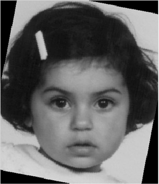
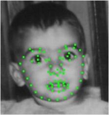
The database we are used is FG-NET(Face and Gesture Recognition Research Network), which is built by the group of European Union project FG-NET who work on face and gesture recognition. This dataset contains 1002 images of 82 subjects whose age varies from 0 to 69. Each image was manually annotated with 68 landmark points located on the face. And for each image, the corresponding points file is available. The figure below shows the sample images and the landmarks on a face image.

Figure 1. A sample from FG-NET with Landmarks

Stage 1: Data Preprocessing

Step I. Image Filtering.

To simplify the processing and enhance the prediction accuracy by the end, we chose only the images in which people faced the camera directly. Images like Figure 2 were not used. At last, we got 617 satisfying images out of the total 1002 images in the dataset.

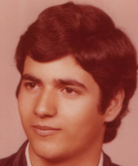
Figure 2. An image sample not been used

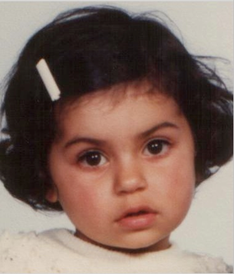
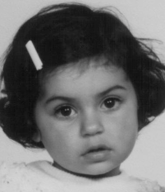
Step II. Image Graying.

Since we need to use the texture on the face as one important feature that predicts the age, we processed all the images into gray scale ones; this is shown in Figure 3.

Figure 3. Image Graying

Step III. Image Rotation.

Each image was rotated until the two eyes reached horizontal; this is shown in Figure 4.

Figure 4. Image Rotation

Step IV. Image Resizing.

Firstly, go through all the coordinates files to find the shortest distance D between two eyes in each image. Then resize all the images until the eye-distance in each image is equal to D.

Stage 2: Feature Extraction

ASM

Active Shape Model is a statistical model-based image search method, which is modeling through the statistics of the same type of the target object images. The main characteristic of ASM is to apply a statistical method to model on a certain category of target images, limiting the feature search results within the range of variation of the model by introducing the prior knowledge of the target object.
ASM is a two-step process, the first step is training model based on the training data. The second step is to take the advantage of the guidance of the training model to search image to get the object shape information. In our project, both the training data and test data are from a data set of correctly annotated images. The 68 landmarks are placed on the same way on each of a training set and it is done manually. The points can represent the boundary, internal features, etc. So we only implemented the first step. By examining the statistics of the positions of the labeled points a “Point Distribution Model” is derived. And we neglect the second step for now. The “Point Distribution Model” gives us the mean positions of the points and a number of parameters (eigenvalues) which control the main modes of variation found in the dataset.
There are three main steps in modeling the data.

1. Choosing the proper contour points.

The data set after the data preprocessing stage has 617 sample images of face and each image is annotated with 68 points on the face.
So we get a matrix named Training Data which contains the coordinate of the points and image information.

2. Aligning the data.

Before PCA is applied, we aligned the vectors a little further by moving the center of the face to a certain position in each image.
After that, we get the new shape vectors:

3. Principle Components Analysis

PCA is applied to the shape vector by computing the mean shape:

And the covariance,

The eigenvalues and eigenvectors of the covariance matrix, represents for the eigenvalues, and is listed in descending order.

Choose the t largest eigenvalues which can explain the 98% of the variance in the training shapes.

So we can get

, and the corresponding eigenvectors,.

After PCA, each shape vector can be written as a linear combination of and:

In the above formula,, which are the shape parameters and the coefficients of the first t models.

AAM

To establish the statistical texture model for reflecting the global texture variation of the faces, Firstly, what we need to do is getting all the pixel grayscale values in the face contour area, which can be regard as extracting the shape-independent texture. And then we use the principle component analysis of the shape-independent texture to modeling.

1.      Texture normalization.

We need to get the grey value of each pixel in the texture image in a fixed sequence to generate a vector  where n is the number of the pixels. To compensate for the illumination, we need to do the texture normalization processing. The so-called normalization is to generate gray vector of zero mean and 1 variance.

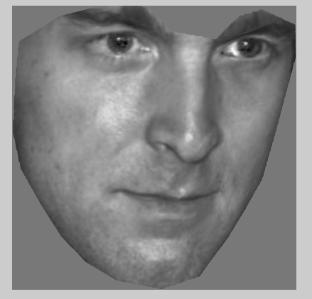
         Figure 5. Example result for texture normalization

2.      Triangulation of the mean shape in shape model.

We introduced Delaunay Triangulation method to divide the mean shape into a collection of triangles.We introduced Delaunay Triangulation method to divide the mean shape into a collection of triangles.

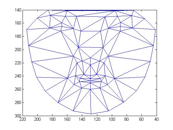
            Figure 6. Result for triangulation of the mean shape

3. Obtaining the shape-independent texture.

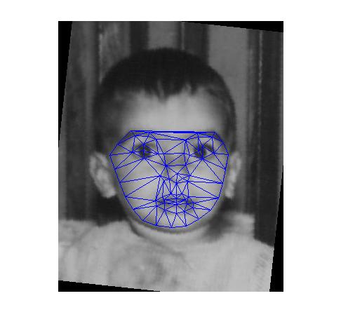
Figure7. Result for triangulation of face sample
Firstly, each face in the training set is deformed into mean shape units each triangle. After triangulation, each face image is composed of a collection of triangular mesh, therefore, by deformation of the shape of each triangle the deformation of whole face image to the mean shape model can be achieved. And by this way, the appearance sample can be obtained in the normal form of mean shape model. Therefore, we can get the shape-independent texture feature.

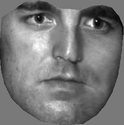
Figure8. Example result for deformation to mean shape

4. Principle Components Analysis.

Like the ASM, AAM also use principle component analysis to build a statistical model of texture. As a result, we can get the eigenvalue, eigenvectors and the mean texture of the appearance model, and after PCA, each shape vector can be written as a linear combination of mean texture and the eigenvectors.

Combination of ASM and AAM

For AAM’s original shape positioning algorithm is not precise enough, ASM cannot take advantage of the texture information, we use a combination of ASM and AAM. After obtaining the shape model and appearance model, each image can be described by a set of texture parameters and shape parameters, because AAM is built based on the shape model, so there is correlation between shape parameters and texture parameters. So it is not proper to combine the models directly, so we combine the two sets of parameters by a weight matrix.
Finally, PCA is used to extract the age feature from the combined model.

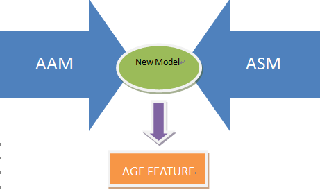
Figure 9. The combination of AAM and ASM

(a)                                              (b)                                              (c)

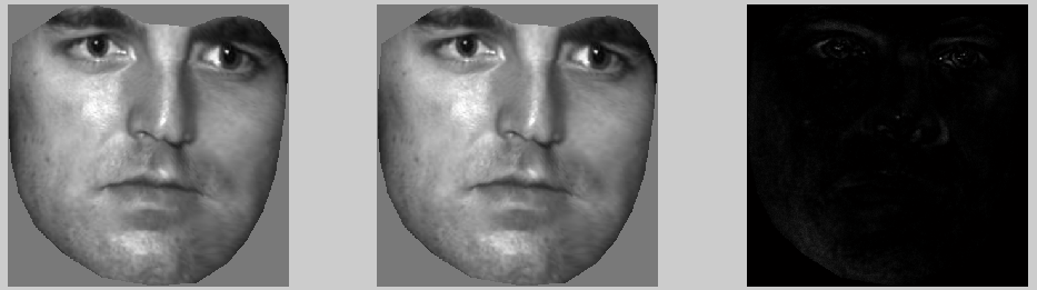
Figure 10. Comparison of original texture with the texture made by combined model.

(a) Original texture. (b) Texture made by the combined model. (c) Difference between original texture and texture described by the combined model.

Stage 3: Training Models and Prediction

Model I. SVR (Support Vector Regression)

Specifically, epsilon-SVR, one kind of SVR, is used to predict the age of a person from one’s face image.

Epsilon-SVR

It introduces parameter epsilon to measure the cost of the errors on the training points. It sets epsilon intensive band to ignore the error of all points that are inside the band.

Figure 11. Non-linear epsilon-SVR

Model II. SVC (Support Vector Classification)

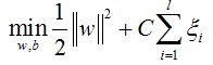In C-SVC, C stands for the parameter in this formula:

At this moment, this is no more than the normal SVM classification method. And it will be optimized for this problem in our future work.

After converting the label to classes index, C-SVC is used to estimate the age range of a person from a face image. The age ranges are 0-5, 5-10, 10-15, ... ,65-70 for the 5-year-a-class model and 0-10, 10-20, 20-30, ... ,60-70 for 10-year-a-class.

Stage 4 Comparing Prediction Errors of Deferent Models

Results:

result for epsilon-SVR

result for C-SVC

To implement C-SVC and epsilon-SVR, the SVM functions Library libsvm^[10]is referenced"

Analysis.

Why is the result of SVR in a sense quite acceptable while SVC performed poorly in this problem? Can we find another way?

The reason is that SVC treats all misclassifications equally while it should not. Apparently, one person of age 12 is more costly to be predicted to be in class 80-90 than in 0-10. Therefore, we plan to add a misclassification error factor to SVC to see if it will enhance the performance of the model and how much is the improvement if exists.

Another way to improve the prediction of SVC is dividing the classification process into 2 parts. The first one tells whether the face belongs to a youth or an adult. In the second phrase, the system will use SVC with different parameters to determine the specific age range.

Future work

1.Cost-Sensitive SVC (as showed at the end of the comparison of SVC and SVR)

2. Two phrases classification (as showed at the end of the comparison of SVC and SVR)

3. Using n-fold or leave-one-out to choose the best values of the parameters for SVR to obtain lower mean square error.

4. If time permits, we will use Matlab to make an GUI application. The expected result is after inputting a picture without any feature points marked, the program can tell the person’s estimated age.

Reference

[1]Xin Geng, Zhi-Hua Zhou, Kate Smith-Miles (2007). Automatic Age Estimation Based on Facial Aging Patterns. Pattern Analysis Machine Intelligence, 29(12), 2234-2240.

[2]Unsang Park, Yiying Tong, Anil K.Jain (2010). Age-Ivariant Face Recognition. Pattern Analysis and Machine Intelligence, 32(5), 947-954.

[3]Ramanathan, N., Chellappa, R., & Biswas, S. (2009). Age progression in human faces: A survey. Visual Languages and Computing.

[4]Steiner, M. Facial Image-based Age Estimation.

[5]Xing Gao. Research on Facial Image Age Estimation.

[6]Hsu, C. W., Chang, C. C., & Lin, C. J. (2009). A practical guide to support vector classification, 2003. Paper available at http://www. csie. ntu. edu. tw/~cjlin/papers/guide/guide. pdf.

[7]Van Ginneken, B., Frangi, A. F., Staal, J. J., ter Haar Romeny, B. M., & Viergever, M. A. (2002). Active shape model segmentation with optimal features. Medical Imaging, IEEE Transactions on, 21(8), 924-933.

[9]Cootes, T. F., Edwards, G. J., & Taylor, C. J. (2001). Active appearance models. Pattern Analysis and Machine Intelligence, IEEE Transactions on, 23(6), 681-685.

[10]Chih-Chung Chang and Chih-Jen Lin, LIBSVM : a library for support vector machines. ACM Transactions on Intelligent Systems and Technology, 2:27:1--27:27, 2011. Software available at http://www.csie.ntu.edu.tw/~cjlin/libsvm